Common challenges and additional resources

Where should you start with a new dataset?

The key to accomplishing any analysis is to start by understand what your data looks like and how it’s organized. This might include:

What type of files are you working with?
How do they get loaded into R?
What is the size of the dataset?
What types of questions can I ask of the data?


library(dplyr)

file <- "/cloud/project/data/single_cell_rna/cancer_cell_id/mcb6c-exome-somatic.variants.annotated.clean.filtered.tsv"
print(file)

# File is a "tsv" file -> Tab-delimited file
read_tsv <- read.csv(file, sep = '\t')

# Look at the file: View(), head(), or click on it to the right
View(read_tsv)
head(read_tsv)

# Understand the variables and data structure: typeof(), str(), colnames()
typeof(read_tsv)
str(read_tsv)
colnames(read_tsv)

Common challenges

NaN and missing data

Dealing with missing data and NaN (Not a Number) values is a common challenge in R programming. These values can affect the results of your analyses and visualizations. It’s essential to handle missing data appropriately, either by imputing them or excluding them from the analysis, depending on the context.

Example:

# Creating a dataframe with missing values
df <- data.frame(
  x = c(1, 2, NA, 4),
  y = c(5, NA, 7, 8)
)

# Check for missing values
sum(is.na(df))


# Understanding missing or sparse information
summary(read_tsv)
read_tsv[!complete.cases(read_tsv),]

Data organization and structure: Factors

Columns that contain strings are automatically read in as character vectors and are arranged alphanumericall. Factors assign a logical order to a series of samples.

file <- "/cloud/project/data/single_cell_rna/cancer_cell_id/mcb6c-exome-somatic.variants.annotated.clean.filtered.tsv"
print(file)

# File is a "tsv" file -> Tab-delimited file
read_tsv <- read.csv(file, sep = '\t')

# Organize the chromosomes to the correct order
# If CHROM is a character vector, the chromosomes are not ordered properly
str(read_tsv) # Shows that CHROM variable is a character vector
ggplot(read_tsv, aes(x = CHROM)) +
  geom_bar() +
  theme(axis.text.x = element_text(angle = 45, hjust = 1))
# make CHROM a factor
read_tsv$CHROM <- factor(read_tsv$CHROM, levels = paste0("chr", c(1:22, 'X','Y')))
str(read_tsv) # shows that CHROM variable is a factor with a set order of character strings
ggplot(read_tsv, aes(x = CHROM)) +
  geom_bar() +
  theme(axis.text.x = element_text(angle = 45, hjust = 1))

Missing packages or dependencies

When running R code, you may encounter errors related to missing packages or dependencies. This occurs when you try to use functions or libraries that are not installed on your system. This will commonly look like a red error stating “There is no package…” Installing the required packages using install.packages(“package_name”) can resolve this issue.

# Trying to use a function from an uninstalled package
library(ggplot2)
ggplot(df, aes(x, y)) + geom_point()
# Error: there is no package called 'ggplot2'

Where do I go for help?

Stack Exchange

Online communities like Stack Exchange, particularly the Stack Overflow platform, are excellent resources for getting help with R programming. You can search for solutions to specific problems or ask questions if you’re facing challenges. If you attempt to Google what you’re trying to accomplish with your dataset, StackExchange often includes responses from others who may have gone through this effort before. With the open crowdsourcing of troubleshooting, these responses that work for others are “upvoted” so that you can try to adapt the code to work for your dataset. Importantly, take care to change the names of variables and file paths in any code that you try to implement from others.

ChatGPT

ChatGPT is an AI assistant that can provide guidance and answer questions related to R programming. You can ask for clarification on concepts, debugging assistance, or advice on best practices. If you copy/paste an error into ChatGPT, it often tries to debug without any other preface. However, if you try to explain exactly what your code is trying to accomplish, it can be a helpful way to debug your help.

Good practices

##Commenting your code Adding comments to your code is crucial for making it more understandable to yourself and others. Comments provide context and explanations for the code’s functionality, making it easier to troubleshoot and maintain.

Publicly accessible resources

Github

Github hosts numerous repositories containing R scripts, packages, and projects. Browsing through repositories and contributing to open-source projects can help you learn from others’ code and collaborate with the R community. This can be a direct way to make your code available upon publication, according to journal practices.

How do I apply the code I’ve learned to my own data?

Once you’ve learned R programming basics, applying the code to your own data involves understanding your data structure, identifying relevant functions and packages, and adapting example code to suit your specific analysis goals.

Additional practice


# Read in the file "/cloud/project/data/bulk_rna/GSE48035_ILMN.Counts.SampleSubset.ProteinCodingGenes.tsv"
# Describe the size, shape, and organization of this data file.


# Example: Applying code to your own data
# Load your dataset
my_data <- read.csv("my_data.csv")

# Explore the structure of your data
str(my_data)

# Identify relevant variables and features
# HINT: Use colnames() and tidyverse functions to clean up your data

# Perform analysis or visualization using appropriate functions and packages
# HINT: Use ggpubr functions to parallelize statistics across groups

# Adapt example code to suit your data and analysis goals
# HINT: Try different methods of plotting. Consider what important features you're trying to understand and show with this data.

# Comment your code for clarity and future reference
# HINT: Make your life easier when it comes time for reproducing your figures and filling in that "Data and Code Availability" section of your manuscript.

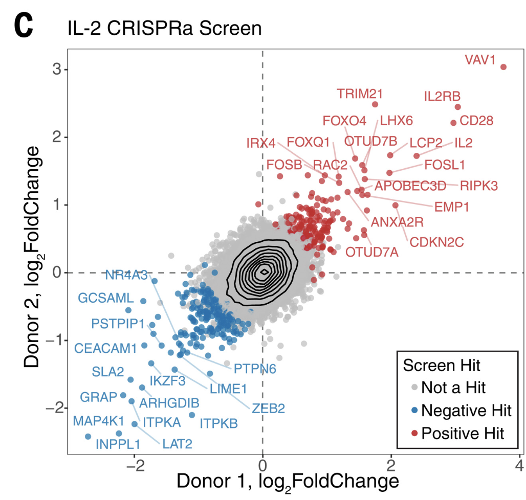
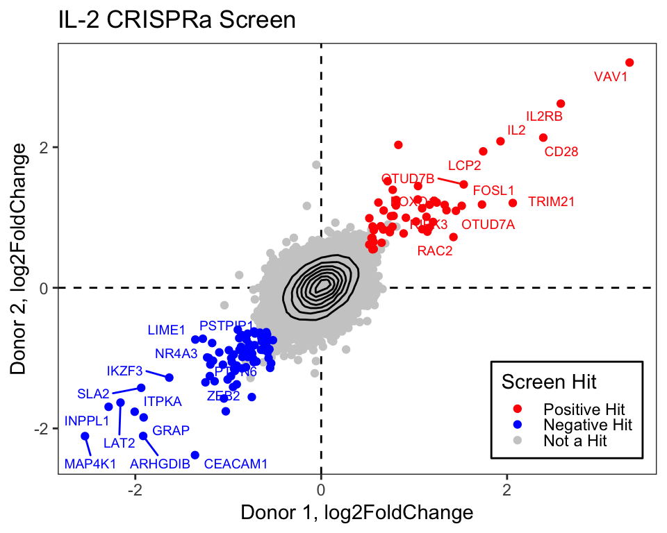
Recreate a Paper Figure from Scratch

Here we will recreate a figure from Schmidt et al (Science 2022):

First we will load the data from the supplemental table (download here):

library(tidyverse)
library(readxl)
library(ggrepel)

log2_df <- read_excel("data/science.abj4008_table_s2.xlsx")

# Always good practice to check the data to ensure it was loaded correctly:
# head(log2_df)

# The plot only contains the IL2 results from CRISPRa screens,
# so we will filter down
log2_df_filter <- log2_df %>%
  filter(Cytokine == "IL2", CRISPRa_or_i == "CRISPRa")

# Select genes that we want to label based on top LFC
ngenes_label <- 16
label_genes <- log2_df_filter %>%
  filter(Screen_Version == "Primary") %>% # For ease only use primary donor
  group_by(sign(LFC)) %>% # Group by the sign (pos or neg) lfc
  arrange(desc(abs(LFC))) %>% # Sort by descending absolute lfc values
  slice_head(n = ngenes_label) %>% # Take the top n genes
  pull(Gene) # Pull these out from the data frame

# We need to pivot the Screen_Version variable (which is equivalent to Donor1 and Donor 2) into separate columns
log2_df_filter_wide <- log2_df_filter %>%
  pivot_wider(id_cols = c("Gene", "Hit_Type"), names_from = "Screen_Version", values_from = "LFC") %>%
  filter(!is.na(Primary), !is.na(CD4_Supplement))


# Reorder the factor so that we can plot the hits on top
log2_df_filter_wide$Hit_Type <- factor(log2_df_filter_wide$Hit_Type,
  levels = c("Positive Hit", "Negative Hit", "NA"),
  labels = c("Positive Hit", "Negative Hit", "Not a Hit")
)


# Now we can plot:
final_plot <- log2_df_filter_wide %>%
  # This will order by the factor so the hits are plotted on top
  arrange(desc(Hit_Type)) %>%
  ggplot(aes(x = Primary, y = CD4_Supplement)) +
  geom_hline(yintercept = 0, linetype = "dashed") +
  geom_vline(xintercept = 0, linetype = "dashed") +
  geom_point(aes(color = Hit_Type)) +
  stat_density_2d(color = "black") +
  # For this geom text, we filter the original data to only include
  # genes that we want labeled from the above filtering
  geom_text_repel(
    data = filter(log2_df_filter_wide, Gene %in% label_genes),
    aes(label = Gene, colour = Hit_Type),
    size = 0.36 * 7, show.legend = F
  ) +
  scale_colour_manual(values = c("Positive Hit" = "red", "Not a Hit" = "grey80", "Negative Hit" = "blue")) +
  theme_bw() +
  theme(
    panel.grid = element_blank(),
    # Place legend inside the plot
    legend.position = c(0.85, 0.15),
    # Change vertical spacing between legend items
    legend.key.height = unit(3, "mm"),
    # Place a box around the legend
    legend.background = element_rect(fill = NA, color = "black")
  ) +
  labs(
    x = "Donor 1, log2FoldChange",
    y = "Donor 2, log2FoldChange",
    title = "IL-2 CRISPRa Screen",
    color = "Screen Hit"
  )
# We can save our plot if desired
ggsave(final_plot, file = "my_pretty_plot.pdf", width = 5, height = 4)

# And now view it
final_plot

Where do I go for practice?

CodeFights

CodeFights (now CodeSignal) offers coding challenges and exercises in R and other programming languages. Practicing coding problems can help reinforce your skills and improve your problem-solving abilities.

Lecture Slides

The slides for this lecture are available here.